Pulling ZIP-Level Census Data in Python
This guide assumes you already have an activated Census API key. If not, start with How to Get a U.S. Census Bureau API Key first.
This is a Python translation of a common R workflow: pulling American Community Survey (ACS) data for a ZIP code and reporting the numbers that matter — for example, how many residents speak Spanish at home and how many have public/Medicaid health insurance coverage, both as raw counts and as a share of the population.
The example below compares two individual ZIP codes. Real projects often group several ZIP codes into custom zones (a school’s enrollment area, a sales territory) — but that grouping logic is a business decision specific to your project, not something a general-purpose tutorial should bake in. Once you can pull and compare two ZIP codes, extending this to grouped zones is a matter of adding your own groupby() on top.
Which Package Should You Use?
In R, tidycensus makes this quick. Two Python options were tested directly against the live Census API before writing this guide:
pytidycensus(the direct port oftidycensus) — its ZIP-filtering option silently ignores the ZIP list and downloads all ~33,800 ZCTAs nationwide every time, regardless of what you ask for. Not usable for this task.censusdis— correctly filters to just the ZIP codes you request, returns an already-numeric DataFrame, and needs only one function call to fetch data. This is what the rest of this guide uses.
pip install censusdis pandas matplotlibIf censusdis won’t install in your environment (its dependency chain — geopandas, Fiona, contextily — can sometimes conflict with other packages in a shared environment like Kaggle), you can hit the Census API directly with requests instead. It’s more code, since you’re doing by hand what the package normally does for you: building the query URL, parsing the raw JSON response, and converting every column from text to numbers.
import requests

codes = list(variables.values())
url = "https://api.census.gov/data/2024/acs/acs5"
params = {
    "get": ",".join(["NAME"] + codes),
    "for": f"zip code tabulation area:{','.join(zips)}",
    "key": API_KEY,
}
data = requests.get(url, params=params).json()

df = pd.DataFrame(data[1:], columns=data[0])
df = df.rename(columns={v: k for k, v in variables.items()})
for col in variables:
    df[col] = pd.to_numeric(df[col])
Everything after this point (summing counts, computing percentages, charting) works identically either way.
Step 1: Define Your ZIP Codes and Variables
Pick the ZIP codes you want to compare, and map readable names to ACS variable IDs:
import censusdis.data as ced
import pandas as pd

API_KEY = "YOUR_KEY_HERE"

zips = ["43035", "43081"]

# ACS 5-Year variable codes
variables = {
    "total_pop":       "B01003_001E",  # Total population
    "female_pop":      "B01001_026E",  # Female population
    "median_age":      "B01002_001E",  # Median age
    "edu_total":       "B15003_001E",  # Population 25+ (education universe)
    "edu_bachelors":   "B15003_022E",
    "edu_masters":     "B15003_023E",
    "edu_prof":        "B15003_024E",
    "edu_doc":         "B15003_025E",
    "race_total":      "B03003_001E",  # Hispanic-origin universe
    "hispanic":        "B03003_003E",  # Hispanic or Latino
    "lang_spanish":    "C16001_003E",  # Speaks Spanish at home (a direct count)
    "medicaid_m_u19":  "C27007_004E",  # Medicaid: Male, under 19
    "medicaid_m_19_64":"C27007_007E",  # Medicaid: Male, 19-64
    "medicaid_m_65":   "C27007_010E",  # Medicaid: Male, 65+
    "medicaid_f_u19":  "C27007_014E",  # Medicaid: Female, under 19
    "medicaid_f_19_64":"C27007_017E",  # Medicaid: Female, 19-64
    "medicaid_f_65":   "C27007_020E",  # Medicaid: Female, 65+
}Table C16001 is easy to get wrong: C16001_002E is “Speak only English” — the exact opposite of what you want. The Spanish-speaker count is C16001_003E. Always verify a variable’s label at api.census.gov/data/2024/acs/acs5/variables/<CODE>.json before trusting it, especially for tables with many similar-looking rows.
Step 2: Fetch the Data
One function call fetches exactly the ZIP codes and variables you asked for, already as numeric columns — no query-building or JSON-parsing required:
df = ced.download(
    dataset="acs/acs5",
    vintage=2024,
    download_variables=["NAME"] + list(variables.values()),
    api_key=API_KEY,
    zip_code_tabulation_area=zips,
)

# Rename columns from ACS codes back to readable names
df = df.rename(columns={v: k for k, v in variables.items()})
This returns one row per ZIP code — no grouping or aggregation needed, since you’re comparing individual ZIPs directly.
Step 3: Read the Counts, Then Derive the Percentages
The number of Medicaid recipients and Spanish speakers are counts you read straight from the report. For Spanish that is a single variable (lang_spanish); for Medicaid you only need to add the six age/sex cells that make up “has Medicaid.” You never compute a count from a percentage.
# Counts, read directly from the report (Medicaid = sum of six C27007 cells):
df["n_spanish"]  = df["lang_spanish"]
df["n_medicaid"] = (
    df["medicaid_m_u19"] + df["medicaid_m_19_64"] + df["medicaid_m_65"]
    + df["medicaid_f_u19"] + df["medicaid_f_19_64"] + df["medicaid_f_65"]
)
df["total_ba_plus"] = (
    df["edu_bachelors"] + df["edu_masters"] + df["edu_prof"] + df["edu_doc"]
)

# Percentages are DERIVED from the counts (count / total population) — not the reverse.
# Dividing every metric by total population makes each one a comparable "% of all residents."
df["Pct_Female"]            = df["female_pop"] / df["total_pop"] * 100
df["Pct_Hispanic"]          = df["hispanic"] / df["race_total"] * 100
df["Pct_Spanish_Speaker"]   = df["n_spanish"] / df["total_pop"] * 100
df["Pct_Bachelors_Plus"]    = df["total_ba_plus"] / df["edu_total"] * 100
df["Pct_Medicaid_Coverage"] = df["n_medicaid"] / df["total_pop"] * 100

result = df[["ZIP_CODE_TABULATION_AREA", "total_pop",
             "n_spanish", "Pct_Spanish_Speaker",
             "n_medicaid", "Pct_Medicaid_Coverage",
             "median_age", "Pct_Female", "Pct_Hispanic", "Pct_Bachelors_Plus"]].round(1)

print(result.to_string(index=False))n_medicaid and n_spanish are counts read straight from the report — the six C27007 cells summed, and C16001_003E as-is. Report the count; then divide by total population if you want a rate. Never do the reverse: multiplying a rounded percentage back by a population to reconstruct a count adds rounding error, and if that population differs from the percentage’s own base, it adds bias too. Counts in, percentages out.
We divide every metric by total population so the percentages are all a comparable “% of all residents.” Some tables have a narrower native universe — C16001 covers only the population 5 and over, and C27007 covers the civilian non-institutionalized population — so if you ever need the exact within-universe rate, divide by that table’s own _001E total instead. For a single comparable base across metrics, total population is the simplest honest choice.
Summing six age/sex cells from table C27007 is the most precise way to isolate Medicaid specifically. If you just need a general “public coverage” percentage (Medicaid + Medicare + VA + other public programs combined) and don’t need the Medicaid-only breakdown, the Data Profile variable DP03_0098PE gives you a pre-computed percentage directly — no summing or division required. Trade precision for simplicity depending on what your analysis needs.
Expected Output
Running the code above against the 2024 ACS 5-year release should produce this table — run it yourself and compare:
| ZIP_CODE_TABULATION_AREA | total_pop | n_spanish | Pct_Spanish_Speaker | n_medicaid | Pct_Medicaid_Coverage | median_age | Pct_Female | Pct_Hispanic | Pct_Bachelors_Plus |
|---|---|---|---|---|---|---|---|---|---|
| 43035 | 36012 | 399 | 1.1 | 2452 | 6.8 | 35.6 | 50.1 | 3.2 | 69.1 |
| 43081 | 65020 | 1253 | 1.9 | 6642 | 10.2 | 36.3 | 52.9 | 3.8 | 54.0 |
And the two headline metrics from this tutorial, visualized:
import matplotlib.pyplot as plt

metrics = ["Pct_Spanish_Speaker", "Pct_Medicaid_Coverage"]
labels = ["Speaks Spanish\nat Home", "Public/Medicaid\nInsurance"]

zip1, zip2 = df["ZIP_CODE_TABULATION_AREA"].tolist()
vals1 = df[df["ZIP_CODE_TABULATION_AREA"] == zip1][metrics].values.flatten()
vals2 = df[df["ZIP_CODE_TABULATION_AREA"] == zip2][metrics].values.flatten()

x = range(len(metrics))
width = 0.32
fig, ax = plt.subplots(figsize=(7, 4.5))
ax.bar([i - width/2 for i in x], vals1, width, label=f"ZIP {zip1}", color="#2a78d6")
ax.bar([i + width/2 for i in x], vals2, width, label=f"ZIP {zip2}", color="#1baf7a")
ax.set_xticks(list(x))
ax.set_xticklabels(labels)
ax.set_ylabel("Percent of Population")
ax.legend()
plt.show()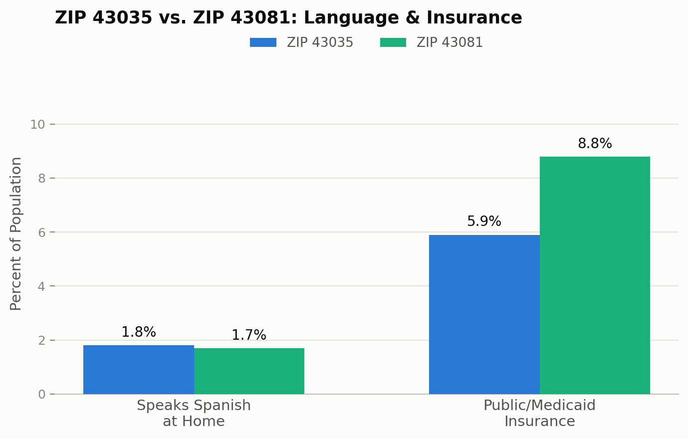
If your numbers don’t match: confirm you’re pulling the same vintage (2024) — ACS estimates shift slightly with each annual data release.
Full Script
Putting it all together:
import censusdis.data as ced
import pandas as pd
import matplotlib.pyplot as plt

API_KEY = "YOUR_KEY_HERE"

zips = ["43035", "43081"]

variables = {
    "total_pop": "B01003_001E", "female_pop": "B01001_026E",
    "median_age": "B01002_001E", "edu_total": "B15003_001E",
    "edu_bachelors": "B15003_022E", "edu_masters": "B15003_023E",
    "edu_prof": "B15003_024E", "edu_doc": "B15003_025E",
    "race_total": "B03003_001E", "hispanic": "B03003_003E",
    "lang_spanish": "C16001_003E",
    "medicaid_m_u19": "C27007_004E", "medicaid_m_19_64": "C27007_007E",
    "medicaid_m_65": "C27007_010E", "medicaid_f_u19": "C27007_014E",
    "medicaid_f_19_64": "C27007_017E", "medicaid_f_65": "C27007_020E",
}

df = ced.download(
    dataset="acs/acs5",
    vintage=2024,
    download_variables=["NAME"] + list(variables.values()),
    api_key=API_KEY,
    zip_code_tabulation_area=zips,
)
df = df.rename(columns={v: k for k, v in variables.items()})

# Counts, read directly from the report:
df["n_spanish"] = df["lang_spanish"]
df["n_medicaid"] = (
    df["medicaid_m_u19"] + df["medicaid_m_19_64"] + df["medicaid_m_65"]
    + df["medicaid_f_u19"] + df["medicaid_f_19_64"] + df["medicaid_f_65"]
)
df["total_ba_plus"] = df["edu_bachelors"] + df["edu_masters"] + df["edu_prof"] + df["edu_doc"]

# Percentages derived from the counts, all over total population:
df["Pct_Female"] = df["female_pop"] / df["total_pop"] * 100
df["Pct_Hispanic"] = df["hispanic"] / df["race_total"] * 100
df["Pct_Spanish_Speaker"] = df["n_spanish"] / df["total_pop"] * 100
df["Pct_Bachelors_Plus"] = df["total_ba_plus"] / df["edu_total"] * 100
df["Pct_Medicaid_Coverage"] = df["n_medicaid"] / df["total_pop"] * 100

result = df[["ZIP_CODE_TABULATION_AREA", "total_pop",
             "n_spanish", "Pct_Spanish_Speaker",
             "n_medicaid", "Pct_Medicaid_Coverage",
             "median_age", "Pct_Female", "Pct_Hispanic", "Pct_Bachelors_Plus"]].round(1)

print(result.to_string(index=False))
Keep Your Key Private
Same rule as always: don’t hardcode your API key in a notebook you’ll share or push to GitHub. Read it from an environment variable instead:
import os
API_KEY = os.environ["CENSUS_API_KEY"]